The purpose of this laboratory exercise is to enhance the skills of learners to observe and calculate the parameters of pulsed signals, to process the data from the measurements and to present the results in appropriate written report.

 

1.     Theoretical introduction.

In this laboratory exercise, signals of interest are pulse shaped voltage and current. The pulse shape is used as baseband in contemporary digital communication equipment and its characteristics are of importance when in exploitation. There are three parameters that define a rectangular pulse:

-         height;

-         width (in time domain);

-         center.

Observing the mentioned parameters, a quantitative analysis of pulses may be made. Three kinds of pulse shapes are the most popular:

-         a rectangular pulse of duration LT (LREC);

-         a raised cosine pulse of duration LT (LRC);

-         a gaussian minimum-shift keying (GMSK).

The mentioned pulse shapes are defined by their amplitude waveform g(t) and by the integral of the pulse form q(t) which stands for “normalized” form. The waveform q(t) can be presented mathematically as:

and the equations, describing the commonly used pulse shapes are:

LREC

 

otherwise
LRC

 

otherwise
GMSK

 
 

The described shapes are depicted on the figures below:

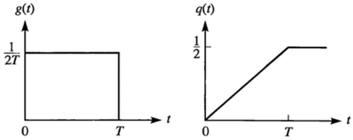
Fig. 1 - A rectangular pulse of duration LT (LREC)

 

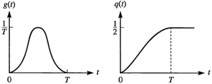
Fig. 2 - A rectangular cosine pulse of duration LT (LRC)

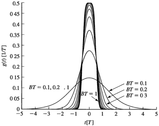
Fig. 3 - A gaussian minimum-shift keying (GMSK)

The coefficient B in GMSK is a bandwidth parameter, which represents the -3dB bandwidthe of the gaussian pulse.

On fig. 4 the main parameters of the pulse shaped signals are shown:

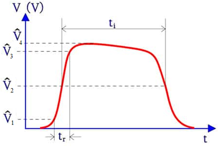
Fig. 4 – Estimation of a rectangular pulse

While on fig. 5 some distortions are grawn.

Fig. 5 – Harmonic distortions on pulse voltage

2.     Practice tasks.

Practice task 2.1: Study the experimental scheme, the principles of pulsed signals measurements and the measurement of parameters and distortions.

To perform a pulsed shape signals measurements, the following equipment is necessary:

-         pulse generator – 1 pcs;

-         timescope meter – 1 pcs.

-         connecting cables and tuples.

Fig. 6 – Pulsed signals measurement scheme

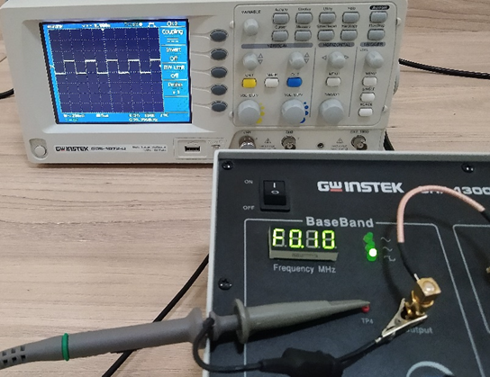
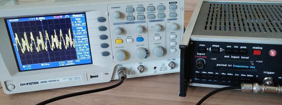
Fig. 7 – A practical realizations of the measurement scheme

 

Practice task 2.2: Measure the amplitude level of a rectangular pulsed signal

This task is done by counting the Y-axis divisions having the units in Volts or Millivolts. Nevertheless, contemporary measurement devices have the ability to calculate the amplitude automatically and it may be shown on the screen.

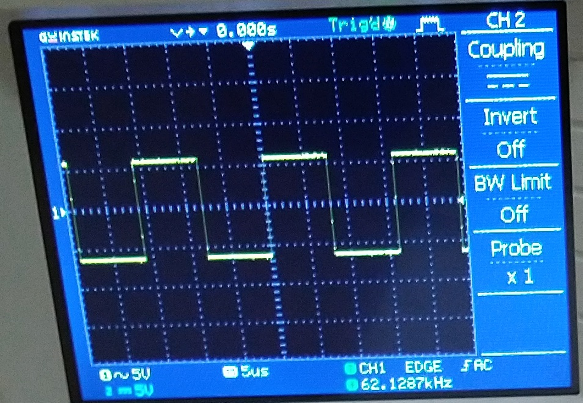
Fig. 8 – Amplitude measurement, 5 V is the Y-axis setting

 

 

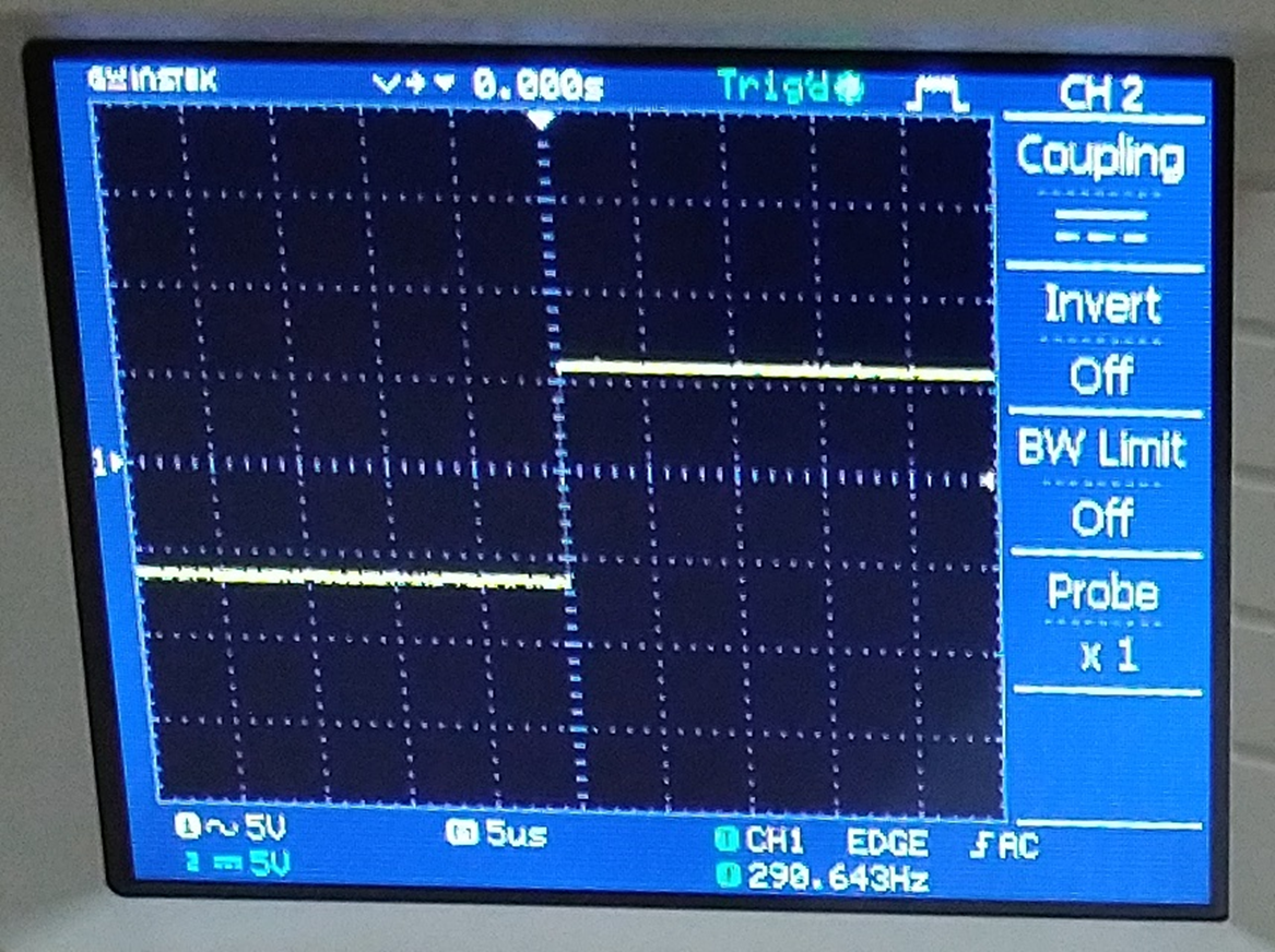
Fig. 9 – Amplitude at 5 µsec trace sweep

 

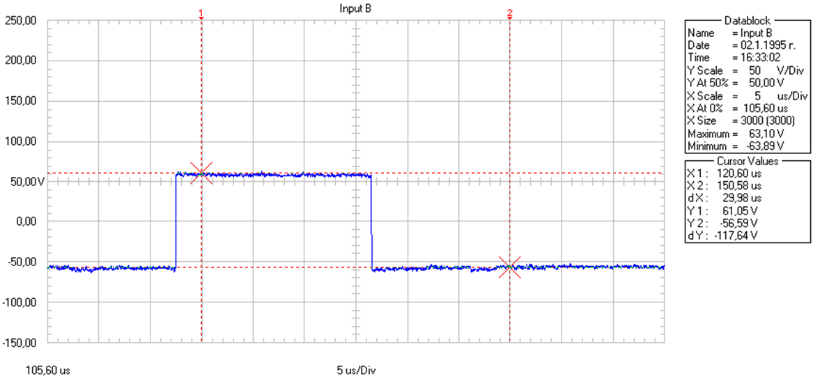
Fig. 9 – Positive amplitude level measurement

 

Fig. 10 – Negative amplitude level measurement

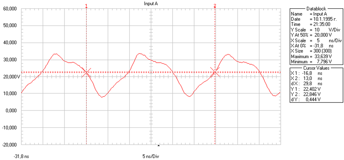
Fig. 11 – Amplitude level measured for 33,639V by the device

 

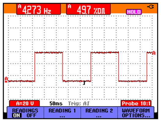
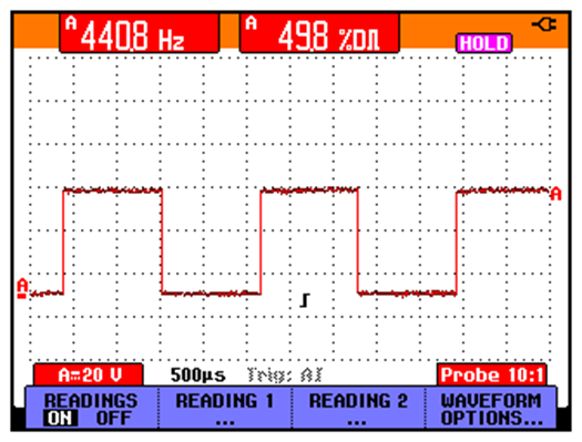
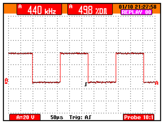
Practice task 2.3: Measure the frequency of pulse shaped signals.

This task can be performed by counting the X-axis divisions of one cycle, or the equipment may show it automatically.

 

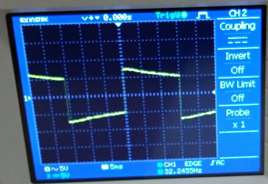
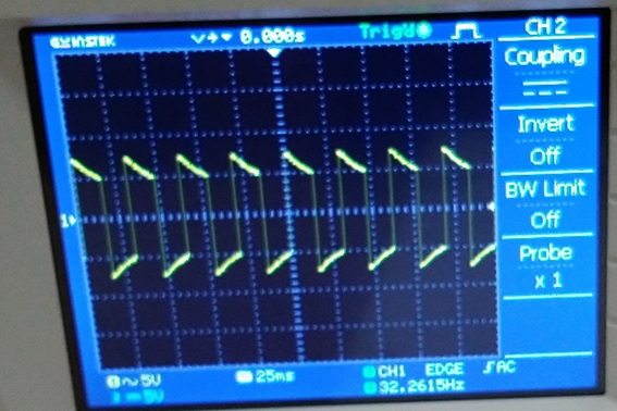
Fig. 12 – Frequency shown to be 32,2455Hz by the device at 5ms and 25ms trace sweep

On fig. 12 shape distortion due to low frequency is seen.

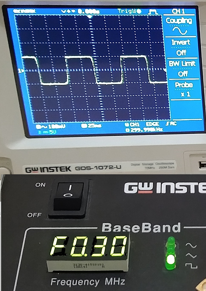
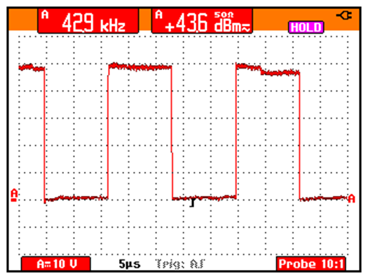
Fig. 13 – 300 kHz transmitted, 299.990 kHz displayed

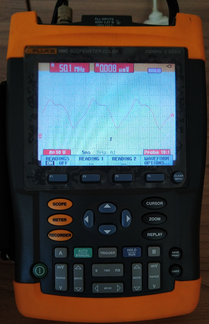
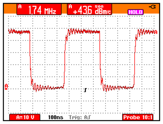
Fig. 14 – 50.1 MHz measured

 

Practice task 2.4: Measure specific parameters.

Depending on the used measurement device, specific parameters may be: Power, Phase offset, Rise time, Fall time, Pulse width, Duty cycle, and etc. An example of measuring the Negative pulse width is shown on fig 15.

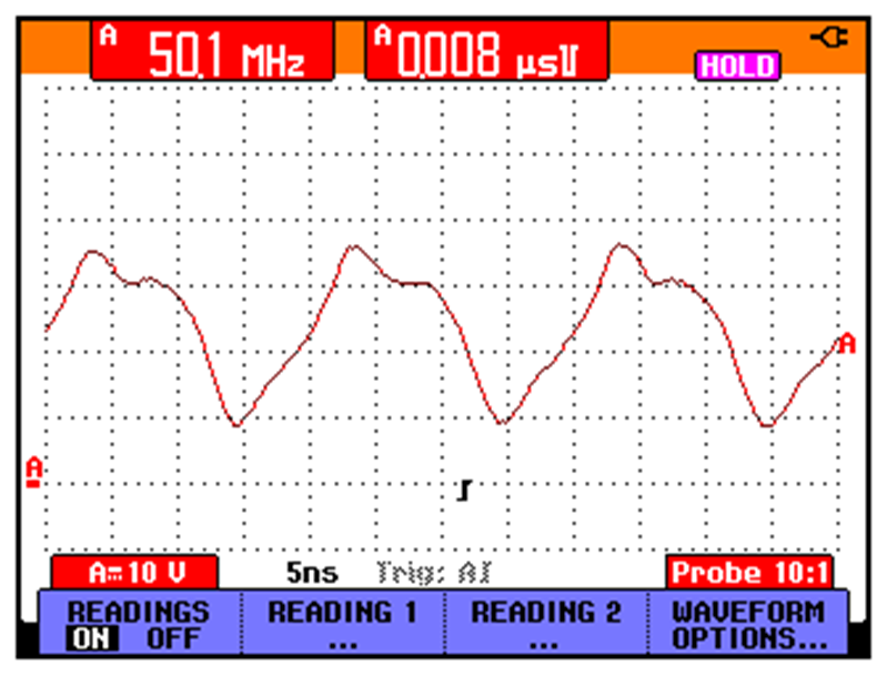
Fig. 15 – Two parameters shown by the device – frequency and negative amplitude pulse width

Measurement of power in dBm:

 

 

Measurement of Duty cycle in the positive semiperiod: