1.      Measurement of time intervals.
1.1         Overview.
Solving many scientific and engineering problems related to the measurement of intervals separating two characteristic moments of a process is an extremely important metrological task. Most often this task is to measure time intervals between two pulse signals.

These measurements are necessary in the sweep and study of various schemes for delay and synchronization, in the study of multi-channel radio systems for time division, in radio telemetry, in radar, in radio control devices, in equipment used in radio physics, nuclear physics, computer technology, etc.

The task of measuring time intervals is important due to the wide use in radio electronics of the conversion of continuous (analog) magnitude into discrete (digital), which is one of the main directions in the sweep of measuring technology. Discrete indicating devices with digital capabilities to measure can be obtained and measuring processes can be automated. It should be emphasized that in many cases the conversion of analog magnitudes into digital code takes place as a result of the intermediate conversion of the tested magnitude over a period of time. The duration of these intervals is in the range of fractions of a nanosecond to units of seconds. Usually the method of comparison (oscillographic) and the method of direct evaluation - the method of discrete counting - are used for their measurement.

1.2         Methods for measuring time intervals.
In practice, two methods are mainly used to measure time intervals: the method of comparison or also known as the sweep method (analog method) and the method for converting the time interval into a digital code (digital method).

1.2.1        Analog sweep methods.
In this method an oscilloscope is used to measure the time interval. Depending on the type of oscilloscope trigger circuit, three measurement methods are used: calibrated linear sweep; linear sweep with calibrated divisions and spiral sweep voltage.

1.2.1.1         Calibrated linear sweep.
Oscilloscopic methods with different types of sweep are very convenient and effective for measuring time intervals with a relatively short duration.

Oscilloscopes designed to measure time intervals in the manner of creating a calibrated linear sweep do not differ significantly from conventional pulse oscilloscopes. The difference consists only in the strictly linear and time-calibrated sweep time or in the stability of the generator for calibrated divisions (Fig. 1).

 

 

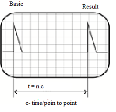
Fig.1

When measuring the time interval between two pulses, the first of them is called reference, and the second - interval. In the case of using a calibrated linear sweep, the reference pulse will trigger the waiting sweep generator and will be fed through the delay line to the vertically deflecting plates. The image of the reference pulse will be obtained at the beginning of the sweep. From the set for fixed calibrated sweeps selects the one in which the two pulses are observed on the oscilloscope screen - the reference and the interval pulses at the maximum distance from each other.

The distance (number of divisions) between them is measured by means of the transparent scale (graticule( in front of the oscilloscope screen , knowing the speed of sweep ( .) The time interval  can be determined.

With this way of measuring time intervals, the sweep must be of very linearity. Otherwise, the measurement errors will due to the incorrectly determined sweep voltage shape (calibration error and non-linearity of the straight beam stroke).

1.2.1.2         Linear sweep with calibrated divisions.
When measuring in this way, a simple linear sweep is used. The time interval is determined by the number of calibrated time divisions or marks on the oscilloscope screen between the image of the reference and interval pulses, analogous to the measurement of the pulse duration in the pulse oscilloscope.

In special oscilloscopes measuring time intervals, high frequency generators are thus used to produce calibrated divisions. This allows the measurement to be performed with high accuracy.

1.2.1.3         Spiral sweep voltage
The use of circular and especially spiral sweep in oscilloscopes significantly increases their resolution, and therefore the accuracy in measuring time intervals. Such sweep can be obtained both for oscilloscopes with ordinary single cathode ray tubes and for cathode ray tubes with an additional conical electrode.

A circular sweep on the oscilloscope screen can be obtained by forming two voltages with equal amplitudes, but out of phase with each other at 900 (Fig. 2).

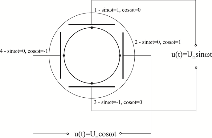
Fig.2

Figure 1, 2, 3 and 4 show the characteristic moments of time of the two stresses and the position of the beam for those moments of time, which clearly represent the way of obtaining a circular sweep.

In order to clarify the method using the spiral sweep, it is expedient to consider the scheme for obtaining such a coil in an electron beam tube with a conical electrode for radial deflection of the beam (Fig.3).

 

 

 

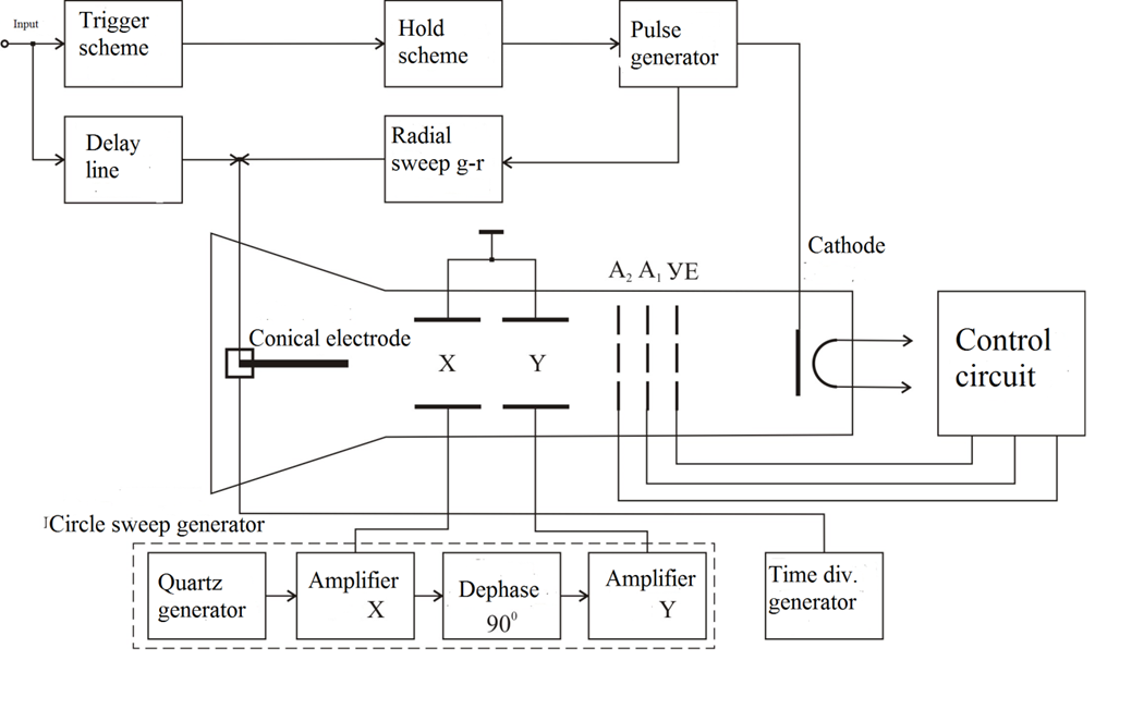
Fig.3

The sinusoidal voltage with frequency  is continuously generated by the quartz oscillator. After pre-amplification, this voltage is applied to the horizontal deflection plates and to the dephasing device, which dephases the signal to 900. After amplifying it by the amplifier in , it is applied to the vertical deflection plates of the cathode ray tube beam on the periphery of the screen. For the specific case, a circle is outlined for time:

 .

Until the arrival of the first pulse (reference) there is no image on the screen, because the tube is blocked by the constant voltage applied to its control electrode. When the reference pulse is received, the pulse generator is activated, which in turn illuminates the screen and activates the radial sweep generator. From the radial sweep generator, the voltage is applied to the conical electrode and causes the beam to deviate from the periphery of the screen to the center. Since the radially deflecting voltage acts simultaneously with the voltage of the circular sweep, the beam will move along the Archimedean spiral - a spiral sweep is obtained.

The reference pulse is fed through the hold line to the conical electrode and causes a radial deflection of the beam. Until the moment of input of the instrument of the interval pulse, delayed with respect to the reference by a certain time (which must be measured), the beam travels a certain distance along the spiral, i.e. the reference and interval pulses can be separated by several turns of the spiral. According to the number of turns of the spiral and the part of the incomplete winding, the time interval between the two pulses can be determined, since the time for which the beam performs one complete circumference is known (one winding fig.4).

 

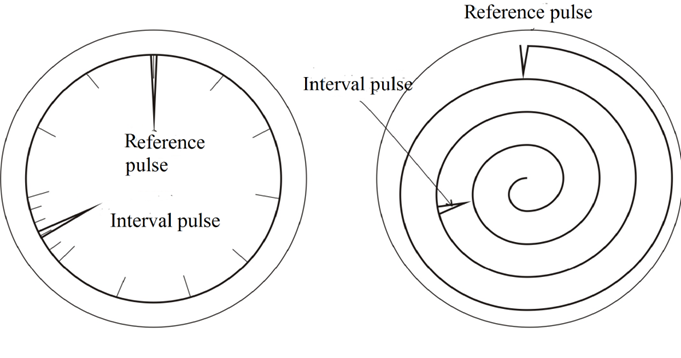
Fig.4

For convenience in measurement and to increase the accuracy of the spiral, calibrated time divisions are applied. They are made of a pulse generator with a short duration and a small amplitude, the frequency of which is a multiple of the sweep frequency (a multiplier is often used). As a result, the divisions will be observed on the screen as a slight displacement of the beam in the radial direction and divide one coil of the spiral into an integer number of divisions. The amplitude of the reference and interval pulse is seen much more clearly against the background of the divisions, because have a larger amplitude.

The oscillograms obtained on the screen of the cathode ray tube can be photographed with a camera with external or internal synchronization. With a photomagnifier (eg aspectomat) when counting the divisions, the time interval can be accurately determined.

1.2.2         Method of converting the time interval into digital code.
The measured time interval  is compared with a calibrated discrete time interval. This is done by filling the measured time interval with pulses having a certain follow-up period   , i.e. by converting the interval into a proportional number of pulses, which are counted by an electronic counter.

The functional diagram of the device with which the method is implemented has the form shown in Fig.5.

 

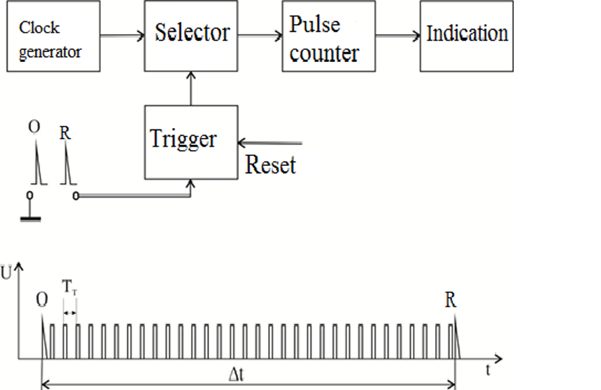
Fig.5

The electronic pulse counter is unlocked and plugged using a timer (selector), which is a circuit with two inputs and one output. The output signal of this circuit has a duration equal to the duration of the pulses acting simultaneously on the input. The clock pulses continuously entering one input of the time selector pass into the pulse counter only when a pulse is received at its second input from the trigger - at a high level of the pulse (1) at the output of the same. Therefore, the input of the clock pulses depends on the state of the trigger. The trigger has two steady states - high output potential (1) and low output potential (0). Therefore, in the initial state, the trigger has a blocked left and unlocked right half (states 1-0, respectively). In this situation, the clock pulses from the generator cannot pass into the electronic counter, because the second input of the timer lacks the required voltage.

When a reference pulse is applied to the input of the device, it will turn the trigger from state 0 to state 1. Its voltage at the output increases sharply. The interval pulse, setting the end of the interval, turns the trigger over again, returning it to the initial position 0. At the same time, the voltage at its output decreases sharply.

In this way, a pulse with steep fronts is formed at the output of the trigger - front and rear and with duration equal to the time of the measured interval. In radio electronics it is accepted to call this impulse gating. Since the gating pulse is fed to the second input of the timer for the time it is unlocked, the clock pulses pass through it, which are counted by the counter. In measuring technology, the gating pulse that sets the duration of the count is commonly referred to as the time gate. The number of pulses fixed by the counter and counted with the numerical indication corresponds unambiguously to the measured time interval.

If the frequency of repetition of the clock pulses of the generator is  (repetition period ), then for the measured time interval  m pulses pass through the time gate.

Therefore, the measured time interval is determined by the ratio:

For convenience in the immediate sampling in seconds, it is advisable to choose a clock frequency , where k = 1, 2, 3, ...

Then the time interval is defined as:

In this way, the duration of a rectangular pulse can also be measured. In this case, the measured pulse must be fed directly to the input of the timer as a gate. The time gate will then have duration .

The conversion of the time interval into a proportional number of pulses can also be done with the help of a generator with shock excitation. For this purpose, a gating pulse with duration equal to the measured time interval is applied to its input. During the operation of the gating pulse, the generator produces  clock pulses. Their number will be a unique function of time, i.e. . It is necessary to determine the error in measuring the time interval by this method.

The error in measuring each quantity by the method of comparison with a sample (reference) quantity consists of:

- Error of the sample (reference) measure;

- Comparison error;

- Error recording and reporting the result.

When measuring a time interval by the method of discrete counting, a sample measure is the frequency of repetition of the clock pulses. Therefore, in the given case, the error of the sample measure will be determined by the instability of the frequency of the clock generator. In time interval meters by this method, the generator is usually quartz stabilized and the input error is usually much smaller than the others. If a shock-induced generator is used, it should be borne in mind that its frequency stability is relatively low and the error of the standard can be significant.

The error of comparison is mainly determined by the conversion of the continuous quantity (time interval) into discrete (number of pulses passed through the time gate) and can be significant. It depends on the mismatch of the moments of occurrence of the clock pulses relative to the front or the decrease of the gating pulse, i.e. they are not synchronized. Therefore the maximum value of the error due to the discreteness of the count is ± 1 of the lower digit of the counter. When an LC-generator with shock excitation is used, the clock pulses are synchronized with the front of the gating pulse. The discretion error in this case can be reduced almost twice and there will always be the same sign. The error of comparison also depends on the accuracy of the timing formation. It should be noted that the use of a trigger with a high rollover speed makes this error practically insignificant. The error of fixing and reading the result of the comparison is irrelevant if the pulse counter has a sufficiently large capacity (volume) and high speed of operation. In other words, if it can capture all incoming impulses, no matter how fast they arrive and regardless of their number. For this purpose, the relationship between the minimum value of the measured value and the relative error due to the discreteness of the method and the speed of the counter will be considered.

If the measured time interval is filled by  clock pulses, then at an absolute error of discreteness ± 1 the relative error will be:

    and,    

and also that the speed of the counter must be greater than the frequency of the clock pulses. Then it turns out:

where  is the speed of the counter.

For example, if the speed of the counter is , then the minimum time interval that can be measured at a sampling error of not more than 1%  will be:

In conclusion, it should be noted that the measurement error will also be affected by noise.

1.2.3        Types of counters.
The pulse counter is an electronic device that registers the number of pulses received at its input. The process of determining this number consists in sequential storage of the value reached so far, the change and the receipt of each subsequent pulse and memorization of the new number. Memorization takes place in separate units (cells) of the counter, each of which can memorize as many different numbers (there are as many different states) as the basis of the counting system used . Triggers or trigger systems with the necessary connections between them are most often used as such units. The number of pulses registered by the counter is determined by the states of the individual triggers, as well as by their consecutive numbering in the circuit forming the counter. Each unit corresponds to a certain digit of the registered number. The first unit they enter the incoming pulses are remembered by the youngest discharge, and the last by the oldest. The registered number will be determined by the expression:

where  are coefficients which, depending on the states of the triggers, can take values

The pulse counting is performed by changing each state of the input pulse by  to the state of the first unit from . This pulse returns the unit to its initial state and this transition is registered as the first pulse in the next unit. Subsequent input pulses again change the state of the first unit from , as the second  pulse sends a signal  from the first to the second unit. When the second unit reaches state , the  received pulse at its input returns it to the output state and sends to the third unit signal , etc.

The main parameters of the counters are:

- Volume (capacity);

- Partition coefficient;

- Resolution time;

- Maximum frequency of the input signal;

- Time to establish.

The volume of the counter is determined by the maximum number of pulses that it can register unambiguously, i.e. , where n is the number of digits of the counter.

After registering the maximum number of pulses, the counter returns to the state from which its action began. In addition, a pulse is generated at the output of its last digit which can be used as the output of the counter. Therefore, if pulses with a repetition frequency are continuously fed to the input of the counter, after each  pulse at its output a series of pulses with a repetition frequency will be obtained:

This allows the counter to be used as a frequency divider with a division factor .

Resolution time  is the minimum time between two consecutive input pulses at which they can be registered by the counter as two. If the interval between them is less than the minimum time, then the second pulse will not be able to activate the counter. Since each unit divides the frequency of the input pulses  times, the resolution time for identical units is determined by the speed of the first cell.

 The maximum frequency of the counter  is the lowest frequency of the input pulses at which each received pulse is registered, i.e. . Since the resolution time is set for two consecutive pulses, the speed will decrease with a continuous series of input pulses due to recharging of any capacities in the counter.

 Settling time is the time from the moment of receipt of the input pulse to the final establishment of the state characterizing the new registered number. That depends on the switching time of the units, the establishment of the number and the structure of the counter. The classification of counters can be done on various grounds:

(a) According to the counting system used.

Binary counters - ). The pulses are registered in a binary number system. They are characterized by the greatest simplicity, but it is difficult to report the results of the count. They are mainly used as counters without indication (for further processing of information) and as frequency dividers.

Decimal counters - . The pulses are registered in a decimal number system. They have a more complex device, but reporting the result is convenient and fast. Most often they are realized on the binary-decimal principle - each unit consists of four triggers, but of the possible 16 states only 10 are used.

Counters with arbitrary division factor. They are binary or decimal counters, which after registering a certain number of pulses (other than 2 or 10) return to the initial state.

b) According to the type of elements used in the counter.

Trigger counters. This is the main type of meters due to the simplicity of the device, low cost and high reliability. The property of the triggers is used, when properly connected, to change their state after each pulse received at their input.

Counters with offset registers. They use shifting registers as separate units, and most often they are connected as circular counters. The advantage of this type of counters is that it is not necessary to use a decoder to indicate the result, and the disadvantage is the large number of triggers needed for counting with the same volume.

Counters using elements with very stable states. These are electronic circuits with very stable states or specially designed electro vacuum devices, combining the counting process with the indication such as decathrons, trochotrons, etc. Due to their extremely complex device, decathron counters have not been widely used, but are promising in terms of their integrated implementation. Such structures are already manufactured by industry. The second type of elements - trochotrons have low security and speed, which together with the high complexity does not allow their widespread use.

c) According to the way the input pulses are registered.

Addition counters. Each input pulse increases by 1 the number registered in the counter.

Subtraction counters. Each input pulse decreases by 1 the number registered in the counter.

Reversible counters. Each input pulse can increase by 1 or decrease by 1 the contents of the counter depending on which of the inputs of the counters

 d) According to the way of impact on the trigger counters of the input pulses.

Asynchronous counters. The switching of the individual triggers is performed not simultaneously, but with a delay due to the switching time of the previous triggers - for counters with direct connection of the triggers - or the time for the signal to pass through a number of logic circuits - for counters with serial transmission. Asynchronous counters have a simple device, but more time to establish.

Synchronous counters. All counter triggers switch simultaneously. This is ensured either by appropriate control of each trigger from its predecessors (counters with direct parallel connection) or by using logic circuits (counters with parallel transmission). With synchronous counters, the setup time is the shortest, but their device is more complicated.

Counters with combined effect. The counter is divided into parts. In each of them, one type of connection is applied (for example, asynchronously), and between them, the other type (for example, synchronously). This seeks a compromise between the complexity of the meter and its settling time They can operate in both summation and subtraction mode.

 

2.      Measurement of high and ultrahigh frequency.
1          

2          

2.1         General information of frequency measurement.
Frequency measurement is one of the important tasks of measuring technology. The devices that measure the frequency of electrical signals are called frequency meters. In modern radio electronics, automation and other related fields of science and technology, signals with different frequencies are used - from infrared to ultra-high.

One of the known frequency classifications is the following:

- Infrared - frequencies below 15Hz;

- Low (sound, acoustic) - frequencies from 15Hz - 20kHz;

- High (radio frequencies) - from 10kHz - 3MHz;

- Ultrahigh - frequencies above 3MHz, the upper limit is constantly increasing.

The wide frequency range implies not only a great variety of measuring equipment, but also methods of frequency measurement. To this should be added the high requirements for measurement accuracy. Modern precision laboratory devices make it possible to measure frequency with an accuracy of 10-7 - 10-8, and “ideal” generators such as cesium or rubidium having an accuracy in the range of 10-11 to 10-13. Low frequencies cannot be measured with such accuracy, but for them this is not necessary because the requirements for them are lower.

In order to perform accurate frequency measurement, it is necessary to have a highly stable standard with which to compare the measuring instruments. Of course, the reference frequency must come from a highly stable (not necessarily electrical) process. In addition, it is necessary for the frequency reference to be reproducible at any time. It follows from the relationship between frequency and period that time standards can be used to construct frequency standards. By determining the reciprocal values ​​of the time standards, the frequency standards are obtained. Closely related to the concept of period and frequency of oscillations is the concept of wavelength. It means the distance over which the oscillation propagates per unit time and is related to the frequency with the dependence .

The wavelength cannot be the main characteristic of the oscillation, because depends on the properties of the environment in which it spreads. That is why frequency measuring instruments, although called wave meters, essentially measure frequency and are graduated in frequency.

There are three main methods for measuring frequency - absolute method, comparison method and resonance method.

In the absolute method, the measurement consists in determining the number of oscillations per unit time ( ). At high frequencies such counting is impossible and therefore the measured frequency is divided many times and the low frequency is subjected to measurement. Until recently, this method was used for measurements only in special laboratories, where special standards are also available.

According to the second method, the measurements are performed by comparing the unknown frequency with a reference one. Used at both low and high frequencies.

The third method is used mainly at high frequencies for fast measurements. It is based on the sharp increase in the amplitude of the signals in the oscillating system when the frequency of the natural oscillations coincides with the measured frequency.

2.2         Frequency measurement methods.
In practice, various methods and devices are used to measure the frequency of electrical signals, given the extremely wide range of measured frequency values. However, they can be grouped into the following methods: direct counting method (direct method); stroboscopic method; comparative method; capacitor charge and discharge method; heterodyne method and resonance method. The features and the principle of measurement according to these different methods, their advantages and disadvantages will be considered separately.

2.2.1         Counting method.
The problem is the inverse of measuring the time between two pulses by way of comparison with a certain interval. The comparison is made by counting the pulses filling the time interval :

.

Suppose there is a certain time interval whose duration is calibrated. If this time interval is filled with pulses following an unknown period , then taking into account the number of pulses falling in the calibrated time interval will be obtained:

 , where

In this way, the frequency of harmonic oscillation can be measured. In this case, it is necessary to pre-convert the harmonic voltage with frequency  ( ) into a periodic sequence of pulses whose position on the time axis corresponds to the points of transition of the harmonic voltage through the axis in one direction. Obviously the frequency of following these pulses will be .

In electronic digital frequency meters, the calibrated interval is . If during this time the - pulse passes, then the average value of the measured frequency will be .

The functional diagram of such a device is shown in Fig.6. The signal whose frequency is to be measured is fed to the input device of the instrument. The forming device converts the sinusoidal voltage of the measured frequency into a sequence of pulses (only with positive or only with negative polarity), the frequency of which is equal to the frequency of the sinusoidal signal. These pulses are fed to one input of the electronic gate (selector). These pulses pass only when the calibrated time gate is open (ie only when a gating pulse of a strictly defined duration acts on the other input).

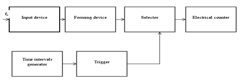
Fig.6

The forming device is performed according to different schemes. The most commonly used amplifier-limiter, which converts the sinusoidal signal into a rectangular one with steep fronts, a differentiating circuit and a one-sided limiter for the formation of short and sharp pulses with a tracking period equal to the period of the studied signal (Fig.7). An asymmetric trigger (Schmidt trigger) is often used to generate rectangular pulses of sinusoidal voltage.

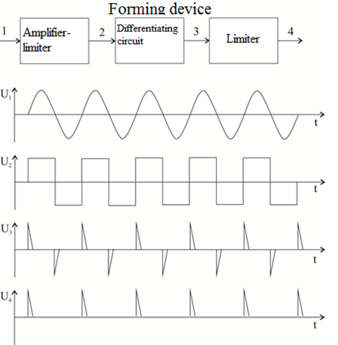
Fig.7

The standard for calibrated time intervals usually consists of a quartz oscillator and a frequency division scheme. In addition, it includes frequency multipliers. The quartz oscillator is a source of high stable frequency oscillations - usually with a frequency of 100 kHz. Some special transmitters can also be used as a frequency reference. The frequency divider circuit is a set of divisors of 10 with a total coefficient - for example 106 - 108. From its output time intervals of 10μs, 100μs, 1ms, 10ms, 100ms, 1s, 10s and 100s can be obtained.

The control device contains a circuit for forming a time interval, a time relay, an indication, a resetting device, a switch of the types of measurements.

The error in measuring the frequency by the method of discrete counting is:

Since the calibrated time interval is set by the quartz oscillator with frequency , the relative error is . The maximum value of the absolute error due to the discrete counting is .

When measuring low frequencies, the error in the discreteness of the count turns out to be decisive and at 10Hz it is 10%. Therefore, low frequencies are measured by electronic frequency meters with relatively low accuracy. There are three ways to increase measurement accuracy:

a). Increasing the duration of the measurement, but this is a significantly inefficient method (a lot of time is lost);

b). Use of frequency multipliers, which reduces the measurement error many times;

c). Rational measurement, i.e. instead of frequency to measure the repetition period.

2.2.2         Stroboscopic method.
The stroboscopic method is used to measure low frequencies. The main element is the stroboscopic disk, on which wreaths are applied, divided into light and dark sectors of equal length. In each subsequent strip, the number of light (and dark) sectors increases by one. The stroboscopic disk is fixed to the axis of a motor that rotates at a constant speed  and is illuminated by a light source powered by a generator of unknown frequency (most often without an inertial lamp). The unknown frequency will be determined by the expression , where is the number of sectors (light only) of the "fixed crown". Higher frequencies can also be measured, but then  - times more sectors should be seen and respectively .

2.2.3        Method of comparison.
The frequency measurement by this method is done according to the connection scheme shown in Fig.8. By changing the reference frequency, equality between the two frequencies X an d  can be achieved. Even higher sensitivity is obtained if the arrow indicator of the beats is turned on.

 

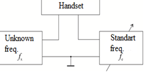
Fig.8

The method of comparing frequencies by means of an oscilloscope using the so-called Lisaju figures is widely used. Frequencies from 10Hz to 10MHz and above can be measured by this method. In this method (Fig. 9) the voltage of unknown frequency is applied to the plates , and the reference frequency of the plates  for horizontal deviation of the CRT (cathode-ray oscilloscope) of the oscilloscope. A fixed figure - a Lisaju figure - is obtained on the screen of the oscilloscope only in cases where the two frequencies are related to each other as two positive integers.

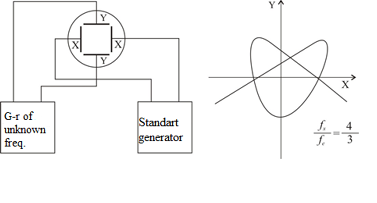
Fig.9

The shape of Lisaju's figures will generally depend on the shape of the voltages, their amplitudes and the ratio of their frequencies and phase differences. In sinusoidal shape and uniform amplitudes, this condition is not mandatory. A crucial condition is that both voltages cause equal deviations along the  and  axes, which can be achieved by correctly selecting the gain in the respective channels. Then the shape will depend only on the ratio of frequencies and phase difference. By adjusting the , a simpler Lisaju figure can be obtained on the screen.

The unknown frequency is determined by the following considerations. For one period of the frequency  the beam moves from the extreme left to the extreme right position and vice versa, i.e. it intersects the  axis twice (or any axis parallel to it). The same applies to the -axis. It follows that if the figure of Lisaju intersects with two lines - one parallel to the horizontal and the other parallel to the vertical axis, then the ratio of the number of points of intersection will be equal to the ratio of the frequencies. A necessary condition is that the lines do not pass through inflex, double and other special points. Fig. 9 shows a specific case for reading the ratio of two frequencies - the known and the unknown.

In practice, the measurement is significantly averaged due to the instability of the reference frequency generators - the figure will change significantly and quickly, especially at higher frequencies and at higher ratios between them.

To measure frequencies with a ratio greater than 10, the method of modulation of some of the parameters of the oscilloscope is used. For this purpose, the generator with frequency  is used to create a circular sweep of the oscilloscope beam by means of a suitably included RC-group (Fig.10).

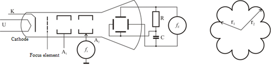
Fig.10

The source of the measured frequency is connected in series to the circuit of the second anode of the CRT of the oscilloscope, i.e. modulation of the sensitivity of the pipe is performed. As a result, the radius of the circle changes from  to  depending on the amplitude of X. A fixed figure is obtained when the ratio  is an integer. Then the number of teeth obtained will determine the relationship between the frequencies. If the ratio is not an integer, then several superimposed figures of "gear circles" will be obtained. In this case, the number of teeth divided by the number of intersections of the line passing through the center (radius) will give us the ratio .

This method, although simple and accurate, is difficult to implement in practice due to the need for high voltage of the signal the frequency at which it will be measured.

The method of image brightness modulation is more widely used. The reference generator is switched on as before, providing a circular sweep of the beam, and the voltage of the measured frequency is included in the circuit of the Venetian cylinder, i. to the modulator (Fig.11). The constant bias voltage is selected so that during part of the period the pipe is unclogged, and during the other part - clogged. Then a broken circle will appear on the screen. The frequency ratio will be determined by the number of light strips. If the assumption that  is not fulfilled, it is necessary to change the switching places of the two frequencies.

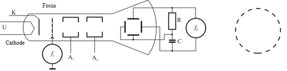
Fig.11

The frequency measurement can also be performed by comparing with the frequency of the linear sweep of the oscilloscope. Moreover, if it is made so that it is  - times lower than the measured one, i.e. , then  - whole periods will be observed on the screen. This method can be used to measure both sinusoidal and non-sinusoidal voltages at   .

The frequency of repetition of the pulse voltages can be determined by applying a reference voltage to the horizontally deflecting plates of the pipe, and the impulse voltage to the vertically deflecting plates. If ,, then a horizontal line will be obtained on the screen and the pulse on it. The same will happen with short frequencies. To avoid this ambiguity, the frequency , is gradually increased from 0 until a pulse is obtained on a straight line. It is then that . In practice, due to the instability of the master generator, the pulse will move.

2.2.4        Capacitor charge and discharge method.
The essence of the method is to measure the discharge current of a capacitor, switched in parallel by a discharge charge with a frequency equal to the measured frequency (Fig. 12).

 

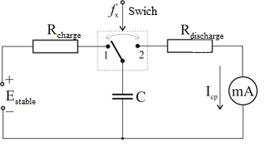
Fig.12

Let capacitor  be charged to voltage  for one half-cycle of unknown frequency and discharged to voltage  for the other half-cycle. Then for one switching of the capacitor from charge to discharge the amount of electricity of the charged capacitor and from it to the measuring instrument will be:

When switching - times per second, the amount of electricity expressed by the current of the measuring instrument will be:

Therefore, the current flowing through the meter is linearly dependent on the switching frequency of the capacitor. An instrument using this method is called a capacitor frequency meter. An electronic switch is used as a switch in it, providing a switching frequency. To ensure a linear dependence of the meter readings on the frequency, a limiter is used that maintains a constant upper charge level of the capacitor. The measuring limits are determined by the size of the capacitor capacity and the sensitivity of the measuring instrument.

Frequency meters in the range from 10Hz to 200kHz (500kHz) work on this principle. The input voltage for this device is in the range of 0.5 to 200V. The main error is ± 1.5% (for the range 200kHz - ± 2%).

2.2.5        Heterodyne frequency meters.
The heterodyne method has become widespread among instruments that allow accurate measurement of frequency. Its essence is in comparison with the measured frequency with the frequency of an adjustable local oscillator. Instruments that use this method are called heterodyne frequency meters, sometimes using the name heterodyne wavemeter.

The operation of the heterodyne frequency meter and the measurement methodology consists of the following (Fig. 13).

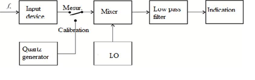
Fig.13

In the  position of the switch, the voltages of the measured frequency and of the local oscillator are applied to the input of the mixer. Voltages with combinational frequencies, including the frequency of zero beats, are obtained at the output of the mixer. The heterodyne will be tuned in frequency until the occurrence of zero (low frequency) beats, fixed by the indicator device. The indicator can be audio (headphones) or visual (indicator lamp, shooting instruments). When zero beats are obtained on the local oscillator scale, the measured frequency will be determined, i.e. then . The accuracy of the measurement depends on the accuracy of the sample measure - in this case on the stability of the frequency generated by the local oscillator, the accuracy of its calibration, as well as on the subjective accuracy in comparing and fixing the zero beats.

To reduce the error of the calibration of the local oscillator in the circuits of many frequency meters, a quartz oscillator is provided, with the help of which the calibration is checked and corrected. This operation should be performed before the start of the measurement. For this purpose, in the  position of the switch, the quartz generator, rich in harmonic oscillations, is connected to the mixer. The scale of the heterodyne is placed at the closest to the quartz harmonic frequency and with the help of a corrector its frequency is changed until the indicator device shows zero beat. If no corrector is provided for the heterodyne generator, its scale is checked in the adjacent two (left and right) frequencies. Linear interpolation is made to introduce a correction. After the correction, the quartz oscillator is switched off and the measured frequency is fed to the mixer. The frequency of the local oscillator will change until zero beats are obtained and the final reading is made on its scale.

At very high frequencies, obtaining and fixing zero beats is very difficult. In this case, a low-frequency frequency meter is switched on instead of an indicator device and the minimum frequency difference is determined.

Due to the presence of higher harmonics in the oscillations generated by both generators (heterodyne and measurements) oscillations will occur not only when the measured and fundamental frequency of the heterodyne generator with smooth tuning, but also when different harmonics are equal. This allows to expand the range of measured frequencies in the field of microwaves, however, uncertainty is introduced in the measurement, as several frequencies will correspond to the same setting position. Therefore, the measured frequency must be known approximately. The frequency measurement methodology depends on the functional diagram of the instrument and will be different for different heterodyne frequency meters.

The industry manufactures and markets about a dozen types of heterodyne frequency meters, covering the frequency range from 100kHz to 80GHz with accuracy classes from 5.10-4 to 5.10-6.

2.2.6        Resonant frequency meters.
One of the most common methods for measuring frequency is the resonance method, based on the use of the phenomenon of electrical resonance in oscillating systems. The essence of this method is concluded in comparison of the measured frequency with the natural frequency of an oscillating circuit or resonator. The method is widely used in high frequency devices and especially in the microwave range. A device that measures frequency by the resonance method is called a resonant frequency meter (often called a resonant wavemeter). The principle of operation of such a frequency meter can be easily explained by the diagram shown in Fig.14.

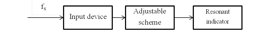
Fig.14

 

The oscillating system is excited by a connection element from the source of the measured frequency. The tuning element changes the natural frequency of the oscillating system until resonance occurs. At the moment of resonance, fixed by the indicator, the frequency of the measured signal is read.

The main element of the wavemeter is the oscillating system. In high-frequency instruments, it consists of a partitioned coil and a precision capacitor with an adjustment scale. The connection between the oscillating circuit of the frequency meter and the source of the measured frequency must be weak, because in case of strong connection:

- The frequency of the generator can be changed;

- The losses in the circle are greater, its characteristic will be flat-tipped and therefore the measurement accuracy is low;

- Due to the large imported resistance, the frequency of the natural oscillations will differ from the frequency of the oscillating circuit graduated for weak connection.

A sure sign of a weak connection between the frequency meter and the signal source is the symmetry of the characteristic of the oscillating circuit.

The connection between the indicator (electronic voltmeter) and the oscillating circuit as a rule does not violate the calibration, but reduces the accuracy of the measurement due to a certain dulling of the maximum characteristic.

Resonant wave meters operate without their own energy source, i.e. they are absorbent - they absorb energy. Therefore, indicators with incandescent, thermocouple, etc. are used when the power of the measured signals is large enough. The indicators with high input resistance - lamp and semiconductor voltmeters, gas discharge lamps, etc. have found wide application.

Coaxial and bulk resonators are most commonly used in the microwave range. The coaxial segment can be half-wave (closed on both sides) or quarter-wave (open on one side). Modern resonant wavemeters use almost exclusively quarter-wave coaxial resonators due to their convenient design and good quality factor.

According to the way of inclusion in the measured circuit, the frequency meters are divided into pass-through and absorbing (reactive). The oscillating system of the pass-through frequency meter has two connection elements - input (1) and output (2). The moment for the setting in resonance is determined by the maximum reading of the indicator (Fig.16). If the oscillating circuit is not tuned to resonance, then the indicator readings will be absent.

 

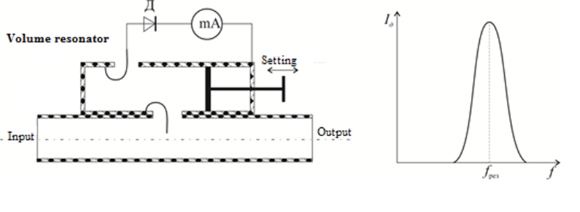
Fig. 16

The absorbing (reactive) wavemeter has only one input and the indicator is connected to the power supply line. As long as the oscillating circuit of the frequency meter is not in resonance, the indicator will show the maximum current. When set in resonance, the oscillating circuit will absorb some of the energy and the indicator readings will decrease. Such a variant for switching on the frequency meter is preferable because it allows continuous monitoring of the operation of the device (Fig.17).

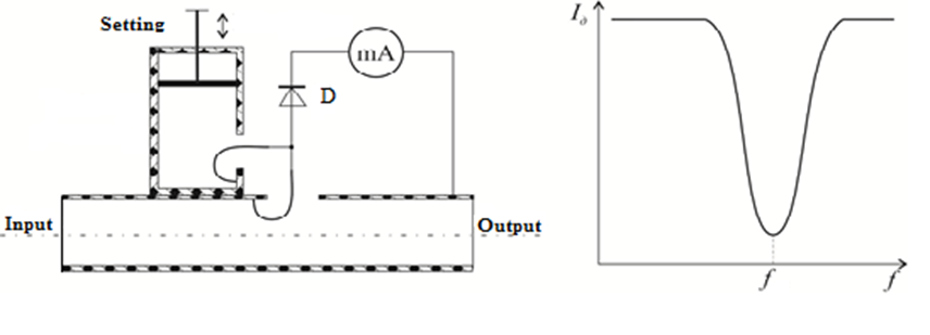
Fig.17

Frequency meters with distributed parameters are connected to the sources of oscillations by means of a stem (whip) or horn antenna. Various coils, probes, slots and holes are used as connecting elements. To reduce the impact of the connection elements at the input and output of the frequency meter, antennas are included. The attenuation introduced by them is usually 10dB. Directional deflectors are sometimes used for connection.

The frequency meter indicator consists of a detector and a magnetoelectric microamperemeter. The connection of the indicator to the oscillating circuit is made in most cases by a connection winding, and the detector is located directly in the electromagnetic field. If the frequency meter is designed to measure frequency in pulse modulation, then a special indicator is needed, containing in its circuit a pulse-extending integrating step, a low-frequency amplifier and a detector voltmeter. External indicators are often used - oscilloscopes or electronic voltmeters, which are plugged into the corresponding socket on the front panel of the frequency meter.