1. Spectrum analysis.

1.1. General information on frequency analysis.

 In 1822, Fourier showed that any complex periodic oscillation can be represented as a simple sum of harmonics (sine and cosine) with different amplitude and certain phase relations between them. The spectral function of the signal is determined by the well-known expression: 

.

 For the pulse shown in Figure 1(a) with values ​​U(t)=U from t= -ti /2 to t=+ti /2 the function is:

 .

After integration, the amplitude-frequency spectrum is:

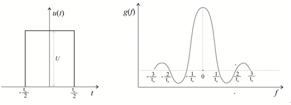
Figure 1

 Figure 1(b) shows the dependence of the amplitude g on the frequency (spectral characteristic). That is the function .

That can be illustrated by the example of how a rectangular or triangular signal can be obtained by summing sinusoids.

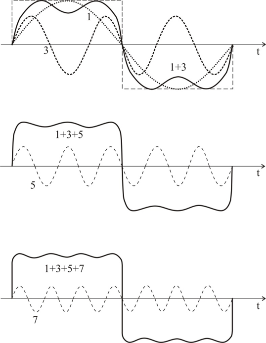
Figure 2

Figure 2 shows the change of a rectangular signal in the presence of odd harmonics (from the first to the seventh).

It can be proved by Fourier analysis that only odd harmonics are needed to obtain a rectangular signal.

Figure 3 shows the formation of triangular voltage by even and odd harmonics.

 

 

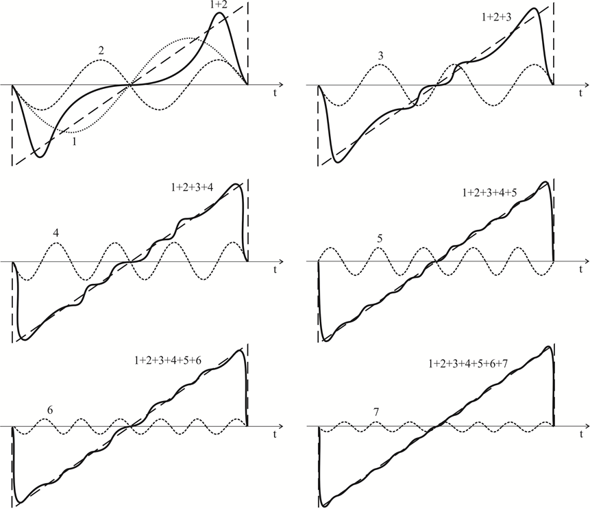
Figure 3

It can be seen from the figure that the greatest voltage linearity is obtained when the signal contains all harmonics (from the first to the seventh inclusive). The cases discussed above show that the analysis of the signal spectrum is of great importance in radio communication systems. In the next question we will consider some methods and equipment for spectrum analysis, which are most used in measurements in radio communication technology.

1.2. Methods of analysis.

Experimental or instrumental analysis of spectra is performed by special measuring devices - spectrum analyzers. With the help of narrowband filters, the corresponding harmonic and its amplitude are determined. There are three possible methods for organizing the analysis:

- Simultaneous (parallel);

- Consistent;

- Combined.

 Simultaneous analysis (parallel) is characterized by the supply of the studied signal in parallel to n narrowband filters tuned to the nth harmonic. A voltage proportional to the amplitude of the corresponding harmonic is obtained at the output of each filter (Fig.4, a). The output signals from the filters can be fed to electronic voltmeters one for each filter. This, of course, is not very economical. More often, the output of each filter is connected in series to the input of an oscilloscope.

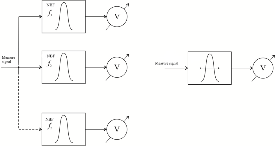
                           a)                                                                                                            b)

Figure 4

The amplitudes of the output voltages from the filters determine the deviation along the vertical axis of the oscilloscope screen. The deviation along the horizontal axis occurs with a voltage proportional to the switching frequency. The advantage of the method is the speed of the analysis. The disadvantage is the complexity of the device that implements it, which consists of adjustable narrowband filters. The sequential analysis is performed using a narrowband filter (Fig.4, b), which has the ability to tune to the required frequency range. It does not have the effect of the parallel method, as the study is performed for each harmonic sequentially over time, adjusting the resonant frequency of the pass filter. Sequential analysis is applicable to the study of processes that change slowly compared to the duration of the analysis. It is inapplicable in its immediate form for the study of fast-moving processes.

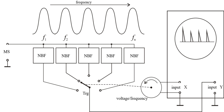
Figure 5

The combined analysis is used to create devices in which the parallel analysis is applied to the subbands, on which the whole frequency range is broken, and within each subband the sequential analysis is applied (Fig. 5).

Spectrum analyzers can be classified:

A) According to the method of analysis: with consistent; with parallel; with combined analysis.

B) By type of indicator: oscillographic; with self-recording devices.

C) According to the frequency range: low frequency; high frequency; ultrahigh frequency.

Spectrum analyzers with sequential analysis have become widespread, in which the "SETUP" process is automated, and the image of the spectrum is observed on the screen, so that the frequencies and amplitudes of the harmonics can be taken into account. Figure 6 shows the block diagram of an oscilloscope spectrum analyzer with automatic adjustment.

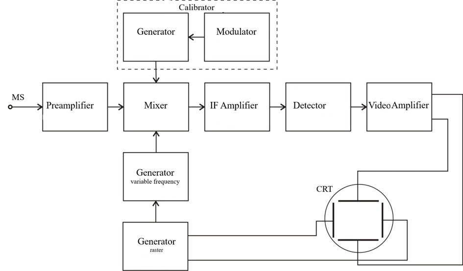
Figure 6

The main unit in this circuit is a super heterodyne receiver consisting of a mixer, a narrowband filter with an intermediate frequency amplifier, a detector, a video amplifier and a variable frequency generator. The diagrams in Fig. 3.25 illustrate the way to obtain a picture of the voltage at the output of the video amplifier.

In the mixer output, a combinational frequency fMX = fMS - fGvf is obtained (along with other combinational frequencies). When it becomes equal to the intermediate frequency fIF to which the selective intermediate frequency amplifier (IFA) is tuned, a maximum gain signal proportional to the amplitude of the input signal is obtained at the output of the IFA. When the combinational frequency is less than or greater than the intermediate frequency, the amplitude at the output of the IFA is correspondingly less or greater, with the amplitude-enveloping curve repeating the resonant curve of the intermediate-frequency amplifier. Thus, in the diagrams of Fig. 7 at time t1, we obtain:

 ,

where: fMS1 is the frequency of the first harmonic of the measurement signal and fG1 is the frequency of generator (VF) signal.

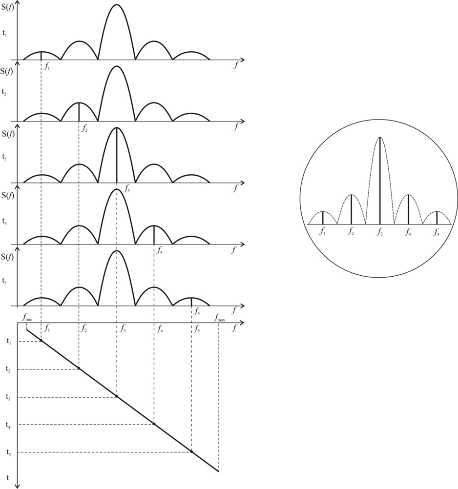
Figure 7

At the moment t2 the condition is:

 

The amplitude of the signal is obtained at the output of the IFA, proportional to the amplitude of the second harmonic, etc. To facilitate the explanation, it is assumed that the development generator controls the movement of the beam in the horizontal direction of the CRT (periodically by linear law over time) and causes a similar law of variation of the frequency of the variable frequency generator (VF). Thus, by converting the spectrum of the probing signal sequentially over time through a single filter operating at a fixed frequency, covering curves with amplitudes proportional to the amplitudes of the studied harmonics are obtained. The detection of the signal thus obtained gives only one polarity of the covering curves, which applied to the vertical plates of the CRT, cause an equivalent deflection of the beam in the vertical direction. Repeating the process with a period of T (usually 20ms, corresponding to the development frequency of 50Hz) causes the appearance of a still image of the curves, which can be taken into account both the amplitudes of the harmonics (vertical axis) and after appropriate calibrations and frequencies them (along the horizontal axis).

2. Amplitude modulation measurement (frequency domain)

The modulated signal can be expressed as below:

Expand this formula with trigonometric expressions to get the next formula:

 

In Fig. 6, a generator with a known frequency is used as a frequency calibrator (the output signal is amplitude modulated). If the modulating voltage is sinusoidal, then the base frequency f0 =2π/ω and the two sideband components, lower sideband f0-Ω and upper sideband f0+Ω are displayed on the oscilloscope screen as vertical stripes against which the base frequency. The amplitude of the upper and lower sideband is equal of MUmax/2. The resulting image is shown in Fig.8.

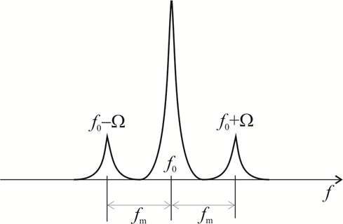
Figure 8

It can be pointed out here that spectrum analyzers can give both the frequency spectrum of the signal and some energy ratios of the components of the frequency spectrum.

3. Frequency modulation measurement (frequency domain)

3.1. Measurement of frequency deviation.

The deviation of the frequency can be most easily measured by the method of the frequency detector. Its essence is that the frequency-modulated oscillations are converted into amplitude-modulated, and then detected by an amplitude detector, resulting in a voltage proportional to the voltage of the modulating frequency. This voltage is measured by a peak voltmeter connected to the output of the amplitude detector. The scale of the peak voltmeter in this case can be directly calibrated in units of frequency deviation, usually in [kHz]. Frequency-modulated oscillations are converted into low-frequency oscillations by a frequency detector (Fig. 9).

The characteristic of the detector uF = φ (Δf) has the form of an S-shaped curve (Fig. 10) and it is called the discriminant characteristic. The details of the frequency detector, especially the oscillating circuits, must be of high quality, as even a small change in their parameters over time will cause a significant change in measurement accuracy.

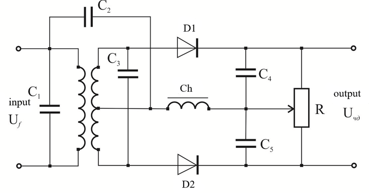
Figure 9

The functional diagram of the device for measuring the deviation by the method of the frequency detector is shown in Figure 10.

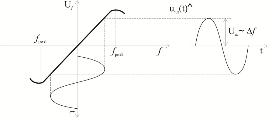
Figure 10

The instrument is essentially a calibrated high-quality heterodyne receiver of frequency-modulated oscillations with measuring instruments for direct reading. The modulated signal is converted to an intermediate frequency, amplified, limited and fed to the input of the frequency detector output voltage, which is proportional to the frequency deviation. The detected voltage passes through a low-pass filter, amplified and measured with a peak voltmeter scale, which is graduated in units of [kHz] for frequency deviation. Check the frequency detector and the entire measuring part of the instrument using an internal calibrator. The measurement error is in the range of ± (5 - 10)%.

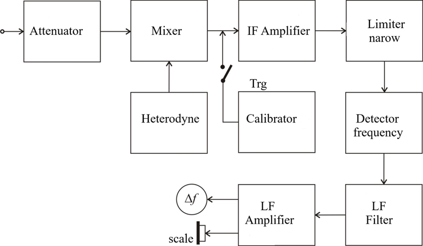
Figure 11

3.2. Measurement of the frequency modulation index.

The analytical expression for frequency modulated oscillation can be represented in spectral form according to the expression:

 where: J0 - Bessel function of the zero order; Jn - Bessel function of the nth order for the harmonics of the signal. The graphs of the frequency-modulated oscillation spectrum for some modulation indices are shown in Figure 12.

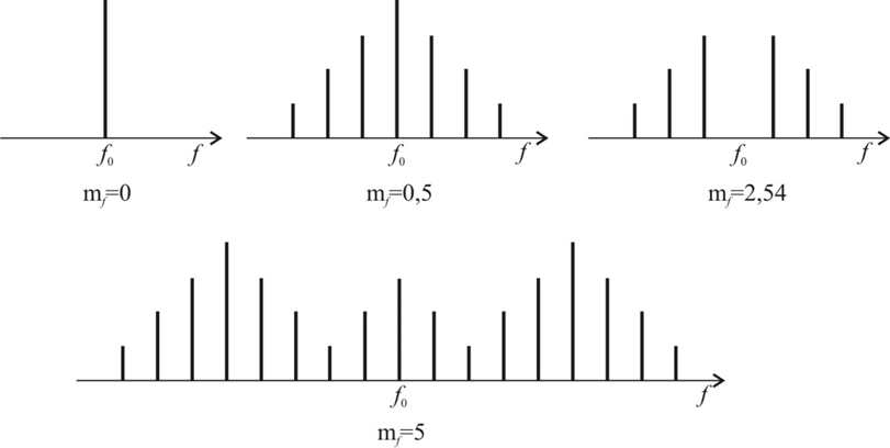
Figure 12

At a certain frequency modulation index in the signal spectrum, the carrier frequency discreteness disappears, which is explained by the fact that the frequency (spectral) representation of the signal is described using a first-order, zero-order Bessel function. The dependence of this Bessel function on the argument mf  is shown in Figure 13. The values ​​of the roots of the Bessel function at certain values ​​of the modulation index mf = 2.4; 5.52; 8.65; 11.79; 14.93; 18.07, etc. become zero, i.e. the carrier frequency disappears from the oscillation spectrum.

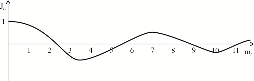
Figure 13

 

 

 

 

Bibliography:

1.     Signal Modulation, J.G. McInerney, in Encyclopedia of Modern Optics, 2005, https://www.sciencedirect.com/topics/physics-and-astronomy/signal-modulation

2.     Modulating Signal, D.I. Crecraft, S. Gergely, in Analog Electronics: Circuits, Systems and Signal Processing, 2002, https://www.sciencedirect.com/topics/computer-science/modulating-signal Processing

3.     Измервания в комуникациите, Т. Г. Пешев, И.А. Илиев, М.К. Киров, НВУ „Васил Левски“, 2017