1. Introduction

Different methods of transmitting useful information are used in the radio transmitting and receiving technology - amplitude modulation, frequency modulation, phase modulation, pulse modulation. In the first three modulation methods, a sinusoidal voltage is used as a signal carrier, while in pulse modulation - a periodic sequence of pulses.

Depending on the shape of the modulating signal, the modulation can be sinusoidal or non-sinusoidal. Discrete modulation (modulation in which the modulating signal is a discrete function of time) is considered as a special case of non-sinusoidal modulation. When considering amplitude, frequency and phase modulation, sinusoidal signal modulation is usually accepted.

Digital modulation is a scheme in which the base-band information has first been converted to a digital message (that is, a message that assumes only one of a finite number of discrete values at a time) before modulation takes place. The digital equivalent of amplitude modulation is amplitude shift keying (ASK), the digital equivalent of frequency modulation is frequency shift keying (FSK), and the digital equivalent of phase modulation is phase shift keying (PSK). In satellite communications PSK is the most commonly used modulation scheme. FSK is occasionally used in applications for which receiver simplicity is a driver.

2. Amplitude modulation measurements. Time domain

Amplitude modulation (AM) is the technique in which the amplitude (peak-to-peak voltage) of the carrier wave is varied as a function of time in proportion to the strength of the data signal.

2.1. Basic relationships.

An electrical signal amplitude modulated with one sinusoidal harmonic is represented as:

                                 

                 (1),

where: Um - amplitude of the unmodulated high-frequency oscillation or carrier signal; f and ω = 2πf - frequency of the carrier signal,; F and Ω = 2πF - frequency of the modulating signal,; M - coefficient of modulation.

The modulation coefficient of the high-frequency oscillation is numerically equal to the ratio of the change of its amplitude ΔUm to the maximum amplitude in the absence of modulation Um:

                                                                                                                                                 (2).

 This ratio is usually expressed as a percentage. The maximum change in amplitude cannot be higher than its value and therefore the maximum modulation coefficient M = 1. In the absence of modulation M = 0. In amplitude modulation, the modulation coefficient and the depth of modulation are the same in both meaning and value.

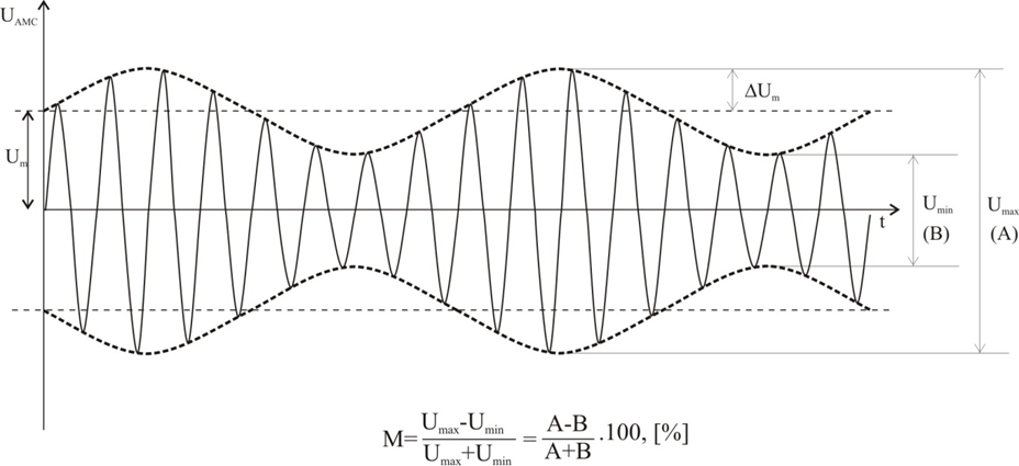
Figure 1

Figure 1 shows the graph of modulated oscillation, from which it follows that:

                                                                                             (3).

The expressions (2) and (3) are true only if the modulation is symmetric. In asymmetric modulation, the expression for M will determine only the average value of the modulation depth.

The effective value of the modulated oscillation is:

                                                                                (4).

Therefore, by measuring with a voltmeter the voltage of the high-frequency non-modulated signal Um and modulated U signal, M can be calculated:

                                                                                                                            (5).

The expression in sqrt changes from 1 to 1.5 when the modulation factor M changes from 0 to 100%. In this case the indication of the voltmeter varies from 1 to 1,225. Therefore, the accuracy of the measurement in this way is worse, especially at small values ​​of M. The amplitude modulation coefficient is determined mainly – oscilloscope method and straightening method.

 2. 2. Oscilloscope method.

Three methods of development can be used to determine the modulation coefficient by the oscilloscope method - linear, sinusoidal and elliptical. In the case of a linear development, the high-frequency modulated signal is fed into the vertical deflection channel, and the frequency of the horizontal scale must be 2-3 times lower than the modulating frequency. The oscillogram of the modulated oscillation (Fig. 1) will appear on the oscilloscope screen in the form U = f (t). By measuring on the scale grid the maximum deviation of beam A = 2Umax and the minimum B = 2Umin is calculated M:

.

To set an oscillogram, the horizontal generator must be synchronized by the modulating signal. The detected modulating signal can also be put into the vertical channel (Fig. 2).

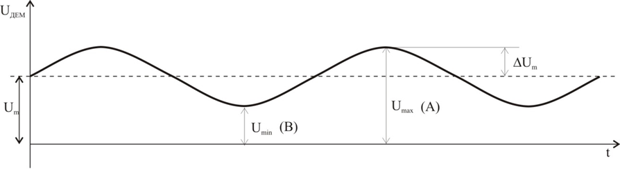
If the oscilloscope is switched for measuring of a DC signal, the oscillogram from Fig.2 will appear on its screen, according to which the modulation factor can be determined. Dimensions A and B are measured using the mechanical scale on the oscilloscope screen. The calculation of the amplitude modulation coefficient is done according to the expression (3).

In the case of a sinusoidal development, the modulated high-frequency oscillation is applied in the vertical channel to determine the modulation coefficient, and the modulating voltage is applied in the horizontal channel. The upper curve of the modulated oscillation causing the beam to deviate in the vertical direction will be determined by the expression:

 .

The deviation in the horizontal direction is obtained as a result of the influence of the modulating voltage:

 .

If (cosΩt) is eliminated from both expressions, Y = Um + Mx will be obtained, and the upper and lower ends of the image will be limited by straight lines, the slope of which will depend on the value of M. On the oscilloscope screen appears oscillogram in the form of a luminous plane with a trapezoidal shape (Fig.3). The lines bounding the plane are Lissajous figures, obtained at the expense of the interaction of the envelopes of the modulated oscillation with the modulating voltage in the absence of a phase difference between them. Dimensions A and B correspond to the maximum and minimum value of the modulated voltage and therefore the modulation coefficient can be calculated by the already known formula for M. If the modulating voltage source is not available, the detected modulating input is put to the horizontal oscillation input of the oscilloscope.

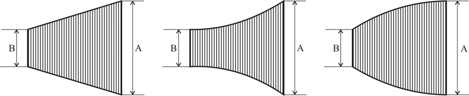
                                  a)                                                               b)                                                  c)

Figure 3

It is preferable to apply the stresses directly to the deflection plates, as the oscilloscope amplifiers will create a certain phase difference and the oscillogram will have a different look. Ellipses will appear here instead of straight, limiting the figure. Such an oscillogram may also indicate that a phase difference occurs in the device under study between the modulating oscillation envelope and the modulating voltage, and nonlinear distortions of the signal occur. The coefficient of modulation is calculated in the same way as before, in which case the dimensions A and B are determined by the tangents to the places of maximum and minimum deviation of the beam. The presence of nonlinear distortions in one of the oscillations or their occurrence in the process of detecting the modulated oscillation is evidenced by an oscillogram similar to that shown in Fig.3, b, c. The value of these distortions on the oscillogram is impossible to determine, only a qualitative assessment is given for the presence or absence of nonlinear distortions. According to the type of the figure obtained on the oscilloscope screen in the absence of distortions and phase difference (Fig. 3.3, a), the method of sinusoidal development is called the trapezoidal method.

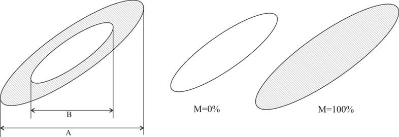
Figure 4

When using an elliptical spreader to determine the modulation factor, the modulated oscillation through a phase-shifting circuit is fed to the two inputs of the oscilloscope with the unwinding generator switched on. A luminous elliptical figure appears on the screen, the internal and external dimensions of which depend on the depth of the amplitude modulation of the measured oscillation (Fig. 3.4). The modulation factor is calculated by the same formula and the dimensions are determined as shown in the figure. The ellipse marked with a single line is obtained in the absence of modulation M = 0%, and the filled ellipse is obtained with a maximum modulation coefficient M = 100%. The oscilloscope method is simple, convenient and clear. It is used in the research or testing of modulated generators or transmitters, when the modulation is performed with sinusoidal voltage in the range of sound frequencies. The carrier frequency is limited by the bandwidth of the amplifiers of the oscilloscope used, and it is therefore best to apply the voltage directly to the deflection plates of the CRT.

The connection of the source of the modulated oscillations to the input of the oscilloscope must be done very carefully. For carrier frequencies below 10MHz, matching does not affect the quality of the waveform. For high frequencies, the length of the connecting wires (lines) must be much less than a quarter of the wavelength. With a large length of the connecting line, its impedance must be at least 10 times less than the reactance of the input capacitance of the oscilloscope. The oscilloscope method can measure the coefficient of modulation from 0 to 100%, as well as demodulation can be observed. The accuracy of the method is low - it depends on the focus of the beam and the accuracy of measuring dimensions A and B. The error can reach 8-10%.

2.3. Straightening method.

 This method is most often used to measure the modulation factor during operation. The essence of the method lies in the fact that the high-frequency modulated oscillation is first detected, and then its constant and variable component is measured. Instruments designed by this method are called modulation meters. Their indicators are usually graduated in percentages of the modulation coefficient M, ie. they turn out to be direct pointing instruments. Depending on the indicators used, the straightening method can be performed in several ways. The most common methods are the square voltmeter and the peak voltmeter. The method with a square voltmeter is realized using the scheme shown in Fig.5 which consists of a diode detector loaded after the filter with two instruments (voltmeters). As a result of the linear detection on the load, a pulsating voltage with low frequency is created, coinciding in shape with the envelope of the modulated oscillation. After the detector, a smoothing U-shaped LC filter is included. The constant component U= corresponds to the carrier frequency voltage. The value of U= is measured by a magnetoelectric voltmeter, protected from the variable component by a choke 

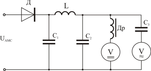
Figure 5

The low frequency AC voltage is measured by the voltmeter results, which correspond to the effective value of the low frequency voltage U~ this voltmeter is blocked by a constant component with the capacitor C3. Therefore, the modulation factor will be equal to:

 .

It is much more convenient to bring the readings of the two voltmeters to the same value at 100% modulation, and by setting the readings of the voltmeter for direct current to some constant "conventional unit", the scale of the voltmeter can be graduated directly in M % ”. It follows from the above expression that it is enough to turn on a transformer or autotransformer with a transformation coefficient of 1.41 before the voltmeter.

3. Measurements in frequency modulation. Time domain.

Frequency modulation systems have very good noise protection and are widely used for high quality radio broadcasting in the VHF range, for the transmission of the audio signal in television systems, radio relay and satellite communication systems. If the modulation is performed with one sinusoidal tone, then the expression for the frequency-modulated oscillation will look like:

 ,

 where: Um - amplitude of high-frequency oscillation; f0 or ω0 = 2πf0 - high (carrier) frequency,; F or Ω = 2πF - frequency of the modulating voltage,; mf - frequency modulation index, determined by the expression:

 ,

 where Δf - high frequency deviation during modulation (frequency deviation).

The instantaneous value of the frequency of the frequency-modulated signal is f = f0 ± Δf. The frequency deviation during modulation is proportional only to the amplitude of the modulating voltage and does not depend on its frequency:

 .

Figure 7 shows the graph of the frequency-modulated oscillation corresponding to the analytical expression. The frequency of the modulating oscillation determines the rate of change of the instantaneous value of the deviation.

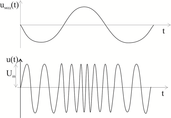
Figure 7

In the practice of radio measurements, especially in operating conditions, the frequency deviation is usually determined. The frequency modulation index for single frequency modulation can be determined if the frequency deviation and the frequency of the modulating voltage are known. For accurate measurement of frequency-modulated oscillations during tuning and calibration of measuring devices, the frequency modulation index mf is determined by measuring the frequency deviation.

Bibliography:

1.     Signal Modulation, J.G. McInerney, in Encyclopedia of Modern Optics, 2005, https://www.sciencedirect.com/topics/physics-and-astronomy/signal-modulation

2.     Modulating Signal, D.I. Crecraft, S. Gergely, in Analog Electronics: Circuits, Systems and Signal Processing, 2002, https://www.sciencedirect.com/topics/computer-science/modulating-signal Processing

3.     Измервания в комуникациите, Т. Г. Пешев, И.А. Илиев, М.К. Киров, НВУ „Васил Левски“, 2017